Nonparametric regression (kernel & Lowess) tutorial

This tutorial will help you set up and interpret a non parametric regression (Kernel / Lowess) in Excel using the XLSTAT software.

What is Kernel regression?

Kernel regression belongs to the family of non parametric regression methods. It is also sometimes related to the smoothing methods. Kernel regression typically requires three phases:

• a fitting step during which one tries to find the best combine of model type, kernel function, and bandwidth, using a test sample.
• a validation phase that allows to validate the model on new observations for which the prediction is known;
• an application phase, where the model is applied to a new set of data for which the prediction is unknown.

Note: nonparametric regression includes a validation phase as a given observation is never used to build the model that is used to generate the corresponding prediction. However, one can still isolate a sub-sample that is only dedicated to the validation phase, to check the model robustness.

On the opposite to the classical linear regression, the goal is not to find a unique model that describes/explains/predict a phenomenon, but to obtain an efficient predictive method. Nonparametric regression is a kind of a black box. It is numerically intensive, as for each observation a new model is computed (in Robust Lowess regression, up to three models are computed for each observation).

Data for the kernel regression

The example that is treated in this tutorial corresponds to a very simple case, and the interest is only illustrative. Nonparametric regression can be very useful to predict complex phenomena such as time series in finance, air pollution from one day to the next, or sales from quarter to the next. It is also sometimes used to smooth a series of data.

The example uses the same data as those used for the tutorial on linear regression .

The data have been obtained in [Lewis T. and Taylor L.R. (1967). Introduction to Experimental Ecology, New York: Academic Press, Inc.]. They concern 237 children, described by their Gender, Age in months, Height in inches (1 inch = 2.54 cm), and Weight in pounds (1 pound = 0.45 kg).

The study is divided into two phases: a fitting phase where 217 individuals are used, and a validation phase with 20 individuals (10 women et 10 men).

Setting up a kernel regression

After opening XLSTAT, select the XLSTAT / Modeling data / Nonparametric regression command, or click on the corresponding button of the Modeling Data toolbar (see below).

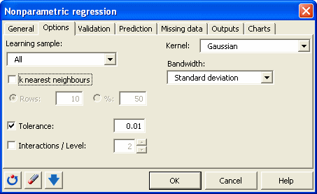
Once you've clicked on the button, the nonparametric regression dialog box appears. You can then select the data on the Excel sheet.

The Dependent variable corresponds to the variable that needs to be explained (or the variable to model), which is here the "Weight".

The explanatory variables are the "Height" and the "Age" (quantitative data) and the sex (qualitative data).

The selection has been done by columns as the data start on the first row. The Variable labels option is activated as the first row corresponds to the name of the variables.

We have chosen to use the polynomial function with degree 1, using All the data (except the one that is being predicted), with a weighting based on the Gaussian kernel, and a bandwidth based on the standard deviation of the variables. The latter allows to avoid scaling effects during the computations.

Note: we are very close to the ANCOVA model, the difference being that we do not use the observation in the model that is used to do the corresponding prediction, and that the weights of the observations in the model depend on their distance to the observation to predict.

The computations begin once you have clicked on OK. The results will then be displayed.

Interpreting the results of a kernel regression

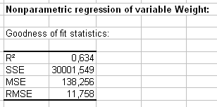
The goodness of fit coefficients allow to evaluate the performance of the model and to possibly compare several models. The R’² (the determination coefficient) gives an idea of the % of the variability of the Weight variable that is explained by the explanatory variables. The closer the R’² to 1, the better the model.

The table of predictions and residuals allows to visualize for each individual the input data, prediction, and the residual. The residuals vary in absolute values between 0.01 (individual 45) and 40 (individual 195). For the validation data that are displayed in the second part of the table, we notice that the residuals vary also a lot. For individuals 229 and 235 the prediction is excellent. It is a lot worse for the individual 224.